Time Series Model(ARIMA) to forecast air passengers in Aviation industry during COVID times

                             

             In light of the rapidly spreading disease named as COVID-19, the International Civil Aviation Organization (ICAO) actively monitoring its economic impacts on civil aviation and regularly publishes updated reports and adjusted forecasts.

The analytical timeframe has now been extended from 2020 to Q1 2021. Let's see what they states:

This shows how covid-19 impacted and hit worst to the aviation industry.

It's crucial to forecast #Passengers would like to travel via flight for the survival of aviation industry. Let's try to predict the passengers about to travel in succeeding months.

I have sample data of passengers travelling between 1949 to 1960. I know, this almost 6 decades old. But, I am just trying to show how time series forecasting methods helps to predict the future and critical to make further business decisions.

Time Series Forecasting divides in 3 major parts:

1. Exploring the data

2. Preprocessing & Estimating

3. Apply Forecasting model

Let's start performing the initial step.🙌 in SAS 

Code:

options validvarname=V7;
proc import datafile='AirPassengers.csv' dbms=csv out=airpassengers replace;


data airpassengers_ts;
set airpassengers;
format Month date9.;
rename _Passengers= Number_of_Passengers Month=Date;

run;

 total observations = 144

/* Stage1 */

title 'Scatterplot Passengers vs. Date'

proc gplot data = airpassengers_ts;

plot Number_of_Passengers*Date;

run;

quit;

The above graphs shows the data is highly non-stationary, variance and mean are not constant. This definitely depicts upward trend.

proc sgplot data = airpassengers_ts;

histogram Number_of_Passengers;

density Number_of_Passengers;

title "Histogram-Density Plot on #Passengers";

run;

The graph looks right-skewed, mean > median. 

proc sgplot data = airpassengers_ts;
series X = Date Y = Number_of_Passengers;
title 'Average quarterly Passengers in Flight';

run; 

This line chart clearly depicts the presence of upward trend. With pace of time, travelers increased. Seasonality also prevails as quarterly, there is change in pattern.

data airpassengers_ts1;

set airpassengers_ts;

Month=month(Date);

Year=year(Date);

run;

proc boxplot data=airpassengers_ts1;

plot (Number_of_Passengers)*Year;

run;

Above Box-Whisker Plot shows the uptrend in number of travelers traveling via flight. In year 1953 becomes turning point in aviation industry. Median > Mean

/* To identify the correlation property, use identity---- nlag=24, bydefault */

proc arima data = airpassengers_ts1;

identify var = Number_of_Passengers nlag=24;

run;

quit;

Let's understand the autocorrelation table to check for White Noise.

In this case, the white noise hypothesis is rejected very strongly, which is expected since the 

series is nonstationary. The p-value for the test of the first six autocorrelations is printed as 

<0.0001, which means the p-value is less than 0.0001.

ACF: A plot of the autocorrelation of a time series by lag is called Autocorrelation Function.
Confidence intervals are drawn as a cone. By default, this is set to a 95% confidence interval, suggesting that correlation values outside of this code are very likely a correlation and not a statistical fluke. Correlation values between 1-15 lags are outside the confidence interval. 
PACF: A partial autocorrelation is a summary of the relationship between an observation in a time series with observations at prior time steps with the relationships of intervening observations removed. 2 & 13 lag shows relationship outside the interval.
ACF & PACF gives intuition about AR and MA in time-series by analyzing these direct and indirect correlations.
This means we would expect the ACF for the AR(k) time series to be strong to a lag of k and the inertia of that relationship would carry on to subsequent lag values, trailing off at some point as the effect was weakened. 
We would expect the ACF for the MA(k) process to show a strong correlation with recent values up to the lag of k, then a sharp decline to low or no correlation.
For the PACF, we would expect the plot to show a strong relationship to the lag and a trailing off of correlation from the lag onwards.

/* Check whether the time-series is stationary or not? */ 

proc arima data = airpassengers_ts1;

identify var = Number_of_Passengers stationarity = (ADF=(1));

run;

quit;

Null Hypothesis : Non-Stationary

Alternative Hypothesis : Stationary

There are three types by which you can calculate test statistics of dickey-fuller test.

Zero Mean - No Intercept. Series is a random walk without drift.

Single Mean - Includes Intercept. Series is a random walk with drift.

Trend - Includes Intercept and Trend. Series is a random walk with linear trend.

Here, p-value > 0.05 which means failed to reject the null hypothesis. The series is non-stationary.

/* Stage 2 */

From the above test, it is clearly signifies the series is not stationary. So to implement forecasting model, it is critical to convert non-stationary series to stationary series.

There are two methods to convert non-stationary series to stationary: Differencing & Detrending.

Below steps will perform differencing. 

proc arima data=airpassengers_ts1;

identify var=Number_of_Passengers(1);

run;

Total observations = 144. By differencing once, then 1 observation will be eliminated. Therefore, now number of observation comes 143.

Still, p < 0.0001. Therefore, series is non-stationary and there is presence of white noise too.

The above ACF shows slight change in series. The series is moving from non-stationary to stationary. Correlation values between 1-7 lags are outside the confidence interval in acf. While, in pacf  correlation values between 1-13 lags are outside the confidence interval.

Let us perform differencing again. 

proc arima data = airpassengers_ts1;

identify var = Number_of_Passengers(2);

run;

quit;

Performing second order differencing, series is not stationary. But in much better position than first order differencing. ACF plot shows there is a presence of MA. We would expect the ACF for the MA(k) process to show a strong correlation with recent values up to the lag of k, then a sharp decline to low or no correlation. 

proc arima data = airpassengers_ts1;
identify var = Number_of_Passengers(1,1);
run;

quit;

Here, First parameter defines differencing the series i.e differencing by lag 1, Second parameter defines removing the observation from seasonality by differencing by lag 1.

ACF & PACF shows variation in plot after differencing by lag 1 on seasonality component.

proc arima data = airpassengers_ts;

identify var = Number_of_Passengers(1,12);

run;

quit;

Here, First parameter differencing by lag 1, Second parameter defines removing the observation from seasonality component by differencing by lag 12. After differencing, the total observations removed from the

series is 13. Due to this, now the series looks stationary. 

Here, p < 0.05 which means the series is devoid of white noise. 

Let's check again whether series is now stationary or not? Perform Augmented Dicker Fuller Unit Testing.

proc arima data = airpassengers_ts1;

identify var = Number_of_Passengers stationarity = (ADF=(1,12,24));

run;

quit;

Examine, Single mean p value. 

For ADF(1) = 0.3240 > 0.05 Therefore, series is not stationary.

For ADF(12) = 0.0010 < 0.05 Therefore, series is stationary.

For ADF(24) = 0.0907 > 0.05 Therefore, series is not stationary.

So, this clearly defines if first order differencing to detrend series and differencing by lag 12 then seasonal components from the series can be removed. This makes the series stationary.

proc arima data=airpassengers_ts1;

identify var=Number_of_Passengers(1,12) minic scan esacf stationarity=(adf=(12,24));

run;

By differencing principle we can remove non-stationary. Proc arima also provides test 
suggestion for p, q values. SCAN or MINIC option in the IDENTIFY statement provide the BIC 
associated with the SCAN table and ESACF table recommendations the p and q values. 

Lower the BIC better is the model.

MINIC STANDS FOR Minimum Information Criterion.

This table provides vital information about best possible P and Q value for the series. 

P=1 & Q=0 gives least BIC value. This makes best fit for the model.

/* To check the presence of Outliers */

proc arima data = airpassengers_ts1;

identify var = Number_of_Passengers(1,12);

estimate P = 1 Q = 0;

outlier;

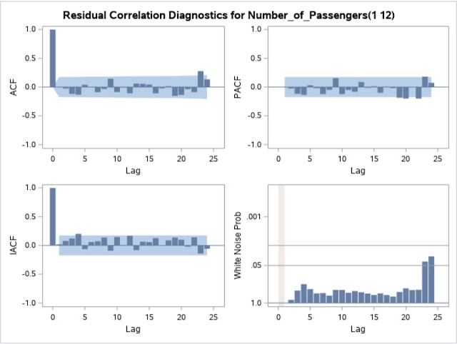
p-value > 0.05. Therefore, there is a presence of residuals in series though it looks stationary. 

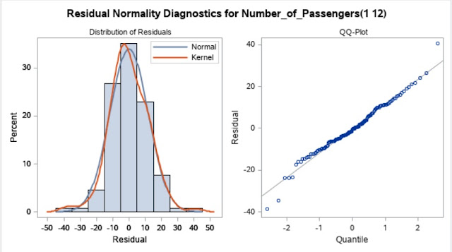
QQ-plot shows linear relation. Deviation is least but there are some outliers in the series and distribution is almost normal.

There are approx. 3 outliers in the series. p<0.05. Therefore, this will not make any significant effect on the model.

/* Stage 3: Forecasting for next 12 observations */

proc arima data = airpassengers_ts1;

identify var = Number_of_Passengers(1, 12);

estimate P = 1 Q = 0;

forecast lead = 12;

run;

quit;

The above table forecast the next 12 observation values ranges within 95% confidence interval.

The above graph forecast the number of passengers in upcoming next 12 months i.e average monthly passengers for year 1961. The value ranges within 95% confidence interval.

Total observation in dataset = 144. Therefore, the next observations named as id from 145 onward.

To forecast the number of passengers for next month after analyzing trends and seasonality in data, applied ARIMA model. This helps in understanding patterns and how likely there is chance of Aviation industry to come out of huge loss. 

Conclusion: 

Understanding the travel history, there seems spike in cherry-blossom around May month. This looks increases till September month. October onwards, number of passengers decreases.

Again in December- January around Christmas & New Year again there is slight increases in rush. 

This looks, people love to travel in hot and humid climate.

From this, we can imagine and remain optimistic about the change in aviation industry on positive note during 2nd Quarter & 3rd Quarter 2021. 

Hope! This article is useful to learn time-series forecasting in SAS and applying ARIMA model.

Happy Learning!💁